Python library Pandas
Pandas is an open source, BSD-licensed library (i.e. module) for providing high-performance, easy-to-use data structures and data analysis tools for Python language. It is used in a wide range of fields involving academic and commercial domains including finance, economics, statistics, analytics, etc.
Pandas library is built on top of Numpy, meaning Pandas needs Numpy to operate. Pandas provide an easy way to create, manipulate and analyze the data.
Data scientists use Pandas for its following advantages:
- It easily handles missing data
- It uses Series for one-dimensional data structure
- It employs DataFrame for multi-dimensional data structure
- It provides an efficient way to slice the data
- It provides a flexible way to merge, concatenate or reshape the data
- It includes a powerful time series tool to work with
In brief, Pandas is a useful library in data analysis. It can be used to perform data manipulation and analysis. Pandas provide powerful and easy-to-use data structures, as well as the means to quickly perform operations on these structures.
In this tutorial, we will learn the various features of Pandas and how to use them in practice using Python.
1) Pandas for Series
We can create a data series from a given array. Then, we can apply various operations on this series. Let us consider the following program to deal with a data series created from a numeric array:
# Example of Pandas Series
import numpy as np
import pandas as pd

# A sample array
data = np.array([11, 22, 33, 44, 55, 66, 77, 88, 99])

# Create series from array
series = pd.Series(data)
print("Full series:~")
print(series, "\n")

# Retrieve the first six elements
print("First 6 elements of series:~")
print(series[:6], "\n")

# Calculate Sum
print("Sum:", series.sum(), "\n")

# Calculate Mean
print("Mean:", series.mean(), "\n")

# Calculate Standard Deviation
val = series.std()
res = format(val, '.2f')
print("Standard Deviation:", res, "\n")

# Use loc() method
print("\n<-- loc -->")
result = series.loc[2:5]
print(result, "\n")

# Use loc() method
print("\n<-- iloc -->")
result = series.iloc[2:5]
print(result, "\n")
Output:
Full series:~
0 11
1 22
2 33
3 44
4 55
5 66
6 77
7 88
8 99
dtype: int32

First 6 elements of series:~
0 11
1 22
2 33
3 44
4 55
5 66
dtype: int32

Sum: 495
Mean: 55.0
Standard Deviation: 30.12

<-- loc -->
2 33
3 44
4 55
5 66
dtype: int32

<-- iloc -->
2 33
3 44
4 55
dtype: int32
2) Pandas for DataFrame
Let us consider this CSV file named “students.csv” denoting a students’ database with the following attributes:
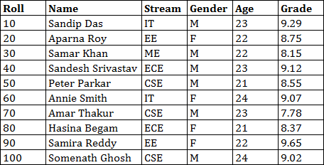
See the example below to create dataframe from the above database and then manipulate & analyze the data in this dataframe:
# Example of Pandas DataFrame
import pandas as pd

# Reading the dataset in a dataframe using Pandas
df = pd.read_csv('students.csv')

# Gathering Info
print('\nInfo of numeric columns: ');
print(df.describe())
# print(df.describe(include="all"))

print('\nInfo of all columns: ');
print(df.columns)
print(df.dtypes)

print('\nSize Info: ');
print(df.shape, "\n")

print('\nBasic Info: ');
print(df.head(10))
# print(df.info) # look at the info of "df"


# df.loc[] gets rows (or columns) with particular labels from the index
print("\n<-- loc 1 -->")
print(df.loc[(df['Grade'] > 8.5), ['Roll', 'Name', 'Stream']])

# df.iloc[] gets rows (or columns) at particular positions in the index (integer value)
print("\n<-- iloc 1 -->")
# DataFrame.values attribute return a Numpy representation of the given DataFrame
print(df.iloc[(df['Grade'] > 8.5).values, [0, 1, 2]])


# Another example of df.loc[] to show it is label-based
print("\n<-- loc 2 -->")
print(df.loc[(df['Grade'] > 9.0) & (df['Stream'] == 'CSE'), ['Roll', 'Name']])

# Another example of df.iloc[] to show it is index-based
print("\n<-- iloc 2 -->")
print(df.iloc[((df['Grade'] > 9.0) & (df['Stream'] == 'CSE')).values, [0, 1]])
Output:
Info of numeric columns:
             Roll        Age      Grade
count   10.000000  10.000000  10.000000
mean    55.000000  22.500000   8.715000
std     30.276504   1.080123   0.569878
min     10.000000  21.000000   7.780000
25%     32.500000  22.000000   8.382500
50%     55.000000  22.500000   8.650000
75%     77.500000  23.000000   9.107500
max    100.000000  24.000000   9.650000

Info of all columns:
Index(['Roll', 'Name', 'Stream', 'Gender', 'Age', 'Grade'], dtype='object')
Roll        int64
Name       object
Stream     object
Gender     object
Age         int64
Grade     float64
dtype: object

Size Info:
(10, 6)

Basic Info:
   Roll               Name Stream Gender  Age  Grade
0    10         Sandip Das     IT      M   23   9.29
1    20         Aparna Roy     EE      F   22   8.75
2    30         Samar Khan     ME      M   22   8.15
3    40  Sandesh Srivastav    ECE      M   23   9.12
4    50       Peter Parkar    CSE      M   21   8.55
5    60        Annie Smith     IT      F   24   9.07
6    70        Amar Thakur    CSE      M   23   7.78
7    80       Hasina Begam    ECE      F   21   8.37
8    90       Samira Reddy     EE      F   22   9.65
9   100     Somenath Ghosh    CSE      M   24   9.02

<-- loc 1 -->
   Roll               Name Stream
0    10         Sandip Das     IT
1    20         Aparna Roy     EE
3    40  Sandesh Srivastav    ECE
4    50       Peter Parkar    CSE
5    60        Annie Smith     IT
8    90       Samira Reddy     EE
9   100     Somenath Ghosh    CSE

<-- iloc 1 -->
   Roll               Name Stream
0    10         Sandip Das     IT
1    20         Aparna Roy     EE
3    40  Sandesh Srivastav    ECE
4    50       Peter Parkar    CSE
5    60        Annie Smith     IT
8    90       Samira Reddy     EE
9   100     Somenath Ghosh    CSE

<-- loc 2 -->
   Roll            Name
9   100  Somenath Ghosh

<-- iloc 2 -->
   Roll            Name
9   100  Somenath Ghosh
I hope that now you have got the confidence of working with Pandas module. This is particularly useful when you will develop solutions for the problems related to data science and machine learning.