Artificial Neural Network (ANN)
Artificial Neural Network (ANN) can perform intelligent tasks similar to the human brain. It is extensively known for exceptional precision and incredible learning capability. ANN also exhibits high tolerance to noisy data. One of the competent methods of data classification from the ANN domain is the Multilayer Perceptron (MLP) neural network. A MLP network is a set of connected input and output nodes with each path having a specific weight. During learning these weights are adjusted so as to classify the correct output from the set of input. Learning is performed on multilayer feedforward neural network by the Backpropagation algorithm. Here, the neural network model learns about a set of weights for a particular predicted class label through iterations.
The network model considers an input layer, one or more than one hidden layer, and an output layer. Each of the layers is built up of nodes. The input to the network corresponds to the attribute present in the training dataset. Inputs are fed into these nodes which make up the input layer. These inputs are then mapped to another level of nodes in the neural network model. This layer is known as hidden layer, the output of this hidden layer can be an input to another hidden layer as illustrated in Figure 1. The number of hidden layer is determined by the complexity of the problem and should be chosen carefully. After the last hidden layer, the nodes are mapped to a set on class labels. This last layer of this model is the output layer of the network, therefore it can be stated that the neural network must contain at least three layers.
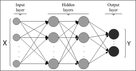
Figure 1: A multilayer feedforward neural network
As shown in Figure 1, the neural network structure appears like a connected graph with each level as a layer in this network with as the input layer and as the output layer. This network is feed-forward as the weight in edges do not cycle back to the input layer or the previous layer. This multilayer feedforward network with sufficient number of given hidden layers can closely predict the values of a function. Before training the network, the study needs to decide the number of nodes for input and output layer and the number of hidden layer(s). Basically, MLP uses Backpropagation technique to build the classification model which is described below.
Backpropagation Technique
This technique learns iteratively from the training data, the neural network is altered for each training tuple to map the test input to an appropriate target value (class label). For each training tuple the weights are modified to reduce mean squared error between the actual result and predicted result. This modification is done backward from the output layer down through the hidden layer to the first layer, thus the name Backpropagation. The steps for learning and testing are described below:
A) Initialization of the weights: The weights in the network are initialized to number within a small interval (for e.g. values within the range -1.0 to +1.0). Each of the nodes in the neural network has a bias associated with it. This bias is also initialized to small random number. The following steps describe the processing of the training tuples.
B) Forward propagation of the inputs: The training tuple is at first fed to the input layer. Each of the attribute corresponds to individual input node. The input passes through this node unchanged i.e., for an input node, its output will be Oj and is equal to the input value Ij. The input and output of each of the nodes in hidden and output layer is then calculated. In each node of the neural network as depicted in Figure 2 has a number of inputs connected to it is coming from the previous layer. Each of the input connection is assigned with some specific weight. To compute net input, a weighted sum is calculated which can be given as:
Ij = ∑i wij Oi + θj ———> (1)
Thus, equation 1 calculates the net input Ij for the node j, having output the previous node i and wij is the weight of the connection. The bias acts as a threshold to vary the activity of the node.
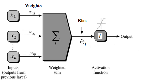
Figure 2: Hidden or output layer of Backpropagation network
Each node in the hidden and output layer takes the calculated net input and applies an activation function to it, shown in Figure 2. This function represents the activation of that neuron which is being represented by that node. The activation function f uses tan sigmoid function. So, the output of the node j can be given as:
Oj = 2.0 / (1 + e-2*Ij ) – 1 ———> (2)
The function as given in equation 2 is also known as squashing function, as it maps the large input domain from the input into a small range of values between 0 and 1. The study computes output values Oj for each of the nodes including the output layer.
C) Propagation of the error: The error that has generated from the network is propagated backward to modify the necessary values to correct the error. For any node j the error Errj can be given as:
Errj = Oj (1 – Oj )(Tj – Oj ) ———> (3)
where Oj is the actual output from node j and Tj is the target known value of the training tuple. Now to compute the error in each hidden layer the study takes Errk as the error of the node in next higher layer k, and then the error in the node j can be given as:
Errj = Oj (1 – Oj )∑k Errk wjk ———> (4)
The weights and bias are updated to correct the errors. The weights are updated according to the following equations:
Δwij = (l)Errj Oi and wij = wij + Δwij ———> (5)
where Δwij is the change in weight and l is the learning rate which varies in between the range -1.0 to +1.0. Similarly, the bias can be modified as:
Δθj = (l)Errj and θj = θj + Δθj ———> (6)
where Δθj is the change in bias. This learning rate is used to avoid getting stuck at a local minimum in decision space. If the learning rate is small, then learning occurs very slowly. If it is too high then it may revolve between insufficient results. Thus, it is a rule to fix the learning rate to 1/t, where t is the current number of iteration completed in training the network.