Cluster Analysis

Clustering is the process of grouping a set of data objects into classes of similar objects. A cluster is a collection of objects that are similar to one another within the same cluster and are dissimilar to the objects in other clusters. Clustering groups objects according to the rule of high intra-class similarity and low inter-class similarity.

To be more specific, one should develop clusters in a manner that the objects belonging to the same cluster have great similarity compared to one another but are very different to the objects in other clusters. Every cluster generated is a group of entities or objects, leading towards the formation of new rules. Clustering is a descriptive data mining task. 

Unlike classification, clustering examines data objects without referring a known class label. The class labels are absent in the dataset as because they are unknown initially. Researchers employ the clustering analysis to create such labels. So, clustering is a form of unsupervised learning technique and is a preprocessing step for classification.

Uses of clustering in real world applications include:

• Customer profiling
• Market segmentation
• Land use
• Search engines
• Astronomy
• Image recognition

Clustering is also called data segmentation in some applications because it partitions large datasets into groups according to their similarity. Cluster analysis can also be used for outlier detection. Applications of outlier detection include the identification of credit card fraudulent activity in e-Commerce applications.

Major Clustering Techniques

The quality of a clustering result depends on both the similarity measure used by the method and its implementation. Major clustering techniques are described below —

1. Partitioning technique:

♦ Create various partitions and then evaluate them by some criterion, e.g., minimizing the sum of square errors

♦ Example methods: k-Means, k-Medoids, CLARANS

2. Hierarchical technique:

♦ Create a hierarchical decomposition of the set data objects using some criterion

♦ Example methods: AGNES, DIANA, BIRCH, ROCK, Chameleon

3. Density-based technique:

♦ Based on connectivity and density functions

♦ Example methods: DBSACN, OPTICS, DENCLUE

4. Grid-based technique:

♦ Based on a multiple-level granularity structure

♦ Example methods: STING, WaveCluster, CLIQUE

5. Model-based technique:

♦ A model is hypothesized for each of the clusters and tries to find the best fit of that model to each other

♦ Example methods: EM, SOM, COBWEB

From the above categories of clustering methods, there is one clustering method that is very popular for its conceptual elegance and simplicity. It is named k-Means which is a partition-based method of clustering. In the next section, this algorithm is described.

k-Means Clustering Algorithm

k-Means is a unsupervised machine learning algorithm. Unlike classification, it examines data objects without knowing the class labels as because they are not present in the dataset. k-Means creates various partitions and then evaluate them by using the concept of minimizing the within-cluster sum of square errors.

The input to this algorithm is the number of data objects present in the dataset (say n) and the number of clusters (say k) to be specified by the user. The output of the algorithm is the set of k clusters resulting in high intra-cluster similarity but low inter-cluster similarity. Cluster similarity is measured with respect to the mean value of the objects in a cluster, which can be viewed as the cluster’s centroid.

The k-Means algorithm proceeds as follows. First, it randomly selects k of the objects, each of which initially represents a cluster mean or center. For each of the remaining objects, an object is assigned to the cluster to which it is the most similar, based on the distance between the object and the cluster mean. It then computes the new mean for each cluster. This process iterates until the criterion function converges.

Given a set of objects (x₁, x₂, …, x_n), where each object is a d-dimensional vector, k-Means clustering aims to partition the n objects into k (≤ n) sets S = {S₁, S₂, …, S_k} so as to minimize the within-cluster sum of squares (WCSS) (i.e. variance). Basically, the objective is to find:

where μ_i is the mean of points in S_i.

Clearly, we can see that WCSS is based on Euclidean distance.

The following pseudocode illustrates the k-Means algorithm for partitioning, where each cluster’s center is represented by the mean value of the objects in the cluster.

k-Means algorithm in pseudocode:

Input: 
    n: the total number of objects
    k: the number of clusters

Output: a set of k clusters 

Method
Initialize k means with random values

Repeat iterating through items:
    Find the mean closest to the item
    Assign item to mean
    Update mean
Until convergence

The method is relatively scalable and efficient in processing large datasets because the computational complexity of the algorithm is O(n∗k∗d∗t), where n is the total number of objects of d-dimensional vectors, k is the number of clusters, and t is the number of iterations needed until convergence (Lloyd’s algorithm).

Numerical Example of k-Means

Problem: Cluster the following eight points with (x, y) representing locations into three clusters A1(2, 10), A2(2, 5), A3(8, 4), A4(5, 8), A5(7, 5), A6(6, 4), A7(1, 2), A8(4, 9). Initial cluster centers chosen arbitrarily are: A1(2, 10), A4(5, 8) and A7(1, 2). Use the k-Means algorithm to find the three cluster centers after the third iteration.

Solution:

The distance function between two points i=(x₁, y₁) and j=(x₂, y₂) based on Euclidean distance is defined as:

d(i, j) = √(|x₂ – x₁|² + |y₂ – y₁|²).

Iteration 1

Based on the distance function, the distance matrix is given below:

∴ New clusters: Cluster 1: {A1}, Cluster 2: {A3, A4, A5, A6, A8}, Cluster 3: {A2, A7}

Next, we need to re-compute the new cluster centers (means). We do so, by taking the mean of all points in each cluster.

For Cluster 1, we only have one point A1(2, 10), which was the old mean, so the cluster center remains the same. So, C1 : (2, 10).

For Cluster 2, we have C2: ( (8+5+7+6+4)/5, (4+8+5+4+9)/5 ) = (6, 6)

For Cluster 3, we have C3: ( (2+1)/2, (5+2)/2 ) = (1.5, 3.5)

The configuration is shown below (in sequence).

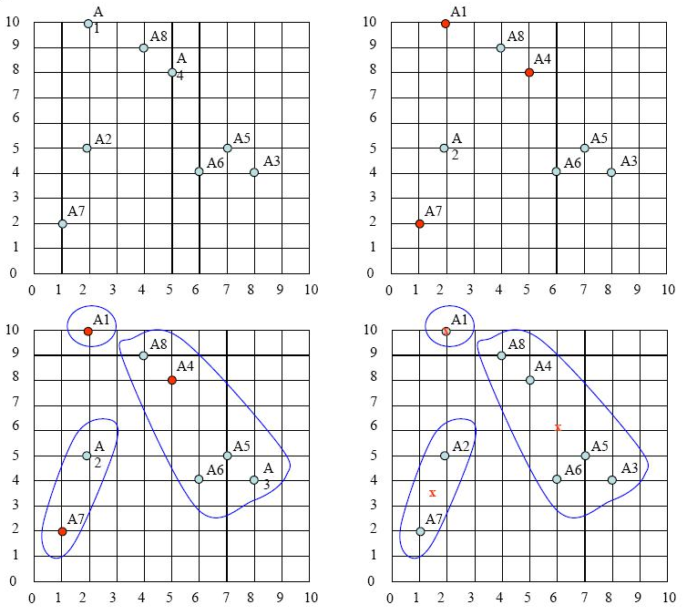
The initial cluster centers are shown in red dot. The new cluster centers are shown in red x.

It was Iteration 1. Next, we go to Iteration 2, Iteration 3, and so on until the cluster means do not change anymore.

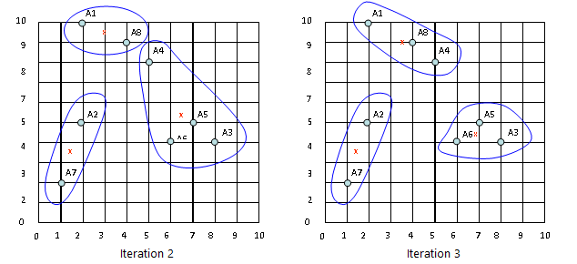
Iteration 2

In Iteration 2, we basically repeat the process from Iteration 1 this time using the new means we computed.

After the Iteration 2, the result would be:

Cluster 1: {A1, A8}, Cluster 2: {A3, A4, A5, A6}, Cluster 3: {A2, A7}

with centers C1=(3, 9.5), C2=(6.5, 5.25) and C3=(1.5, 3.5).

Iteration 3

After the Iteration 3, the result would be:

Cluster 1: {A1, A4, A8}, Cluster 2: {A3, A5, A6}, Cluster 3: {A2, A7}

with centers C1=(3.66, 9), C2=(7, 4.33) and C3=(1.5, 3.5).

The configurations for Iteration 2 and Iteration 3 are shown below together.

Requirements of Clustering in Machine Learning

1. Scalability – One needs highly scalable clustering algorithms to deal with large databases.

2. Ability to deal with different kind of attributes – Algorithms should be capable to be applied on any kind of data such as interval based (numerical) data, categorical, binary data.

3. Discovery of clusters with attribute shape – The clustering algorithm should be capable of detect cluster of arbitrary shape. The should not be bounded to only distance measures that tend to find spherical cluster of small size.

4. High dimensionality – The clustering algorithm should not only be able to handle low- dimensional data but also the high dimensional space.

5. Ability to deal with noisy data – Databases contain noisy, missing or erroneous data. Some algorithms are sensitive to such data and may lead to poor quality clusters.

6. Interpretability – The clustering results should be interpretable, comprehensible and usable.

In the next tutorial, I will provide Python code implementation of the k-Means algorithm using some real world dataset.