Association Rule Mining (ARM)
Association rule mining (alternatively known as frequent pattern mining) is an important machine learning technique. The frequent patterns are patterns that occur in a data set regularly. Given a set of objects or items, for instance, bread, butter and milk that frequently occur together in a supermarket transaction record called a frequent itemset. Discovering these types of frequent patterns plays a vital role in mining relationships among data. Additionally, the procedure can be used for classification, clustering analysis, and other types of machine learning tasks. It is a descriptive data mining technique.
Association rule mining (ARM) denotes the procedure of determining captivating and unforeseen rules from vast databases. The field indicates a very general model that helps in finding the relations between items of a database. An association rule is an if-then-rule supported by data. Initially, the association rule mining algorithms used for solving the market-basket problem. The problem was like this: given a set of objects and large amount of supermarket transaction records, the goal was to find associations between the objects confined to several transactions.
A typical association rule resulting from such a research study can be “60 percent of all consumers who purchase a personal computer also buy antivirus software” – which reveals a very useful information for business. So, this analysis can provide new understandings of customer behavior and thereby leading to higher profits via better customer dealings, customer retaining and better product settlements. The mining of association rules is a field in data mining that has received a lot of attention in recent years. The main association rule mining algorithm, Apriori, not only influenced the association rule mining community, but it affected other machine learning fields as well.
Terminologies
The major aim of ARM is to find the set of all subsets of items or attributes that frequently occur in many database records or transactions, and additionally, to extract rules on how a subset of items influences the presence of another subset. ARM algorithms discover high-level prediction rules in the form: IF the conditions of the values of the predicting attributes are true, THEN predict values for some goal attributes.
Now before describing the association rule and the terminologies related to ARM such as support, confidence and frequent itemset, we need to consider the following basic definitions:
Definitions
- I={i1, i2, …, in}: a set of all the items
- Transaction T: a set of items such that T ⊆ I
- Transaction Database D: a set of transactions
- A transaction T ⊆ I contains a set X ⊆ I of some items, if X ⊆ T
- A set of items is referred as an itemset. A itemset that contains k items is a k-itemset.
Association Rule
In general, the association rule is an expression of the form X⇒Y, where X, Y ⊆ I. Here, X is called the antecedent and Y is called the consequent. Association rule shows how many times Y has occurred if X has already occurred depending on the minimum support (s) and minimum confidence (c) values.
Let us describe the terminologies related to ARM —
Support: The support of an itemset X is the probability of transactions in the transaction database D that contain X:
support(X) = count(X) / N –––> (1)
where ‘N‘ is the total number of transactions in the database and count(X) is the number of transactions that contain X.
The support of the rule X⇒Y in the transaction database D is the support of the itemset X ∪ Y in D:
support(X⇒Y) = count(X ∪ Y) / N –––> (2)
=> Support measures how often the rule occurs in the dataset.
Confidence: The confidence of the rule X⇒Y in the transaction database D is the ratio of the number of transactions in D that contain X ∪ Y to the number of transactions that contain X in D:
confidence(X⇒Y) = count(X ∪ Y) / count(X) = support(X ∪ Y) / support(X) –––> (3)
It is basically denotes a conditional probability P(Y|X).
=> Confidence measures the strength of the rule.
Frequent Itemset: Let A be a set of items, D be the transaction database and s be the user-specified minimum support. An itemset X in A (i.e., X ⊆ A) is said to be a frequent itemset in D with respect to s, if support(X) ≥ s.
The problem of mining association rules can be decomposed into two sub-problems:
Step 1: Find all sets of items (itemsets) whose support is greater than the user-specified minimum support, s. Such itemsets are called frequent itemsets.
Step 2: Use the frequent itemsets to generate the desired rules. The general idea is that if, say ABCD and AB are frequent itemsets, then we can determine if the rule AB⇒CD holds by checking the following inequality:
support({A,B,C,D}) / support({A,B}) ≥ c
where the rule holds with confidence c.
It is easy to find that the set of frequent sets for a given T, with respect to a given s, exhibits some important properties–
♦ Downward Closure Property: Any subset of a frequent itemset is a frequent itemset.
♦ Upward Closure Property: Any superset of an infrequent itemset is an infrequent itemset.
The above properties lead us to two important definitions–
♦ Maximal frequent set: A frequent itemset is a maximal frequent itemset if it is a frequent itemset and no superset of this is a frequent itemset.
♦ Border set: An itemset is a border set if it is not a frequent itemset, but all its proper subsets are frequent itemset.
Therefore it is evident from the above two dentitions that if we know the set of all maximal frequent sets, we can generate all the frequent itemsets. Alternatively, if we know the set of border sets and the set of those maximal frequent itemset, which are not subsets of any border set, then also we can generate all the frequent itemsets.
Apriori Algorithm
The main association rule mining algorithm, Apriori, was proposed by R. Agrawal and R. Srikant in 1994 for boolean association rules. The name of the algorithm is based on the fact that the algorithm uses prior knowledge of frequent itemset property which states that all nonempty subsets of a frequent itemset must also be frequent. This property is also known as the Apriori property.
This is also called the level-wise algorithm, makes use of a bottom-up search, moving upward level-wise in the lattice. This algorithm uses two functions namely candidate generation and pruning at every iteration. It moves upward in the lattice starting from level 1 till level k, where no candidate set remains after pruning.
Essentially, a frequent set is a set of frequent itemsets of size k having a support count value greater than equal to a user-specified minimum support (known as Lk). The candidate set is a set of candidate itemsets of size k called a potentially frequent itemset (known as Ck).
The following pseudocode describes the Apriori algorithm for discovering frequent itemsets:
// Pseudocode of Apriori algorithm
Iteration 1
   1. Create the candidate sets in C1
   2. Preserve the frequent sets in L1

Iteration k
   1. Create the candidate sets in Ck from the frequent sets in Lk-1

      a)Join p ∈ Lk-1 with q ∈ Lk-1, as follows:
        Add to Ck
        select p.item1, p.item2, . . . , p.itemk-1, q.itemk-1
        from p ∈ Lk-1, q ∈ Lk-1
        where p.item1 = q.item1, . . . p.itemk-2 = q.itemk-2, p.itemk-1 < q.itemk-1

      b)Create all (k-1)-subsets from candidate sets in Ck

      c)Prune all candidate sets from Ck where some (k-1)-subset
        of the candidate itemset not present in frequent set Lk-1

   2. Scan the database to determine the support for each candidate set in Ck

   3. Preserve the frequent sets in Lk
Illustration of the working of Apriori Algorithm
Let us solve some problems related to Apriori algorithm.
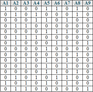
Problem 1: Consider the transaction database, D, which contains 15 records.
The set of items, A = {A1, A2, A3, A4, A5, A6, A7, A8, A9}.
Assume s = 20%. Illustrate the working of Apriori algorithm for the database D.
Solution:
Since s = 20% and D contains 15 records.
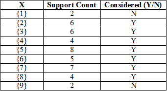
So, minimum support count value is = (15×20)/100 = 3.
k := 1
Read the support count of all 1-itemsets.
The frequent 1-itemsets and their support counts are given below:
L1 := {{2} → 6, {3} → 6, {4} → 4, {5} → 8, {6} → 5, {7} → 7, {8} → 4}
k := 2
In the candidate generation step, we get
C2 := {{2,3}, {2,4}, {2,5}, {2,6}, {2,7}, {2,8}, {3,4}, {3,5}, {3,6}, {3,7}, {3,8},
{4,5}, {4,6}, {4,7}, {4,8}, {5,6}, {5,7}, {5,8}, {6,7}, {6,8}, {7,8}}.
Read the database to count the support of the elements (in bold font) in C2 to get
L2 := {{2,3} → 3, {2,4} → 3, {3,5} → 3, {3,7} → 3, {5,6} → 3, {5,7} → 5, {6,7} → 3}
while the rest of the elements are pruned as they are not considered to be frequent 2-itemsets.
k := 3
In the candidate generation step,
using {2,3} & {2,4}, we get {2,3,4}
using {3,5} & {3,7}, we get {3,5,7} and
similarly from {5,6} & {5,7}, we get {5,6,7}.
C3 := {{2,3,4}, {3,5,7}, {5,6,7}}.
The pruning step prunes {2,3,4} as not all subsets of size 2, i.e., {2,3}, {2,4}, {3,4} are present in L2.
Thus the pruned C3 is {{3,5,7}, {5,6,7}}.
Read the database to count the support of the elements in C2 to get
L3 := {{3,5,7} → 3}.
k := 4
Since L3 contains only one element, C4 is empty and hence the algorithm stops, returning the set of frequent sets along with their respective support values as
L := L1 U L2 U L3
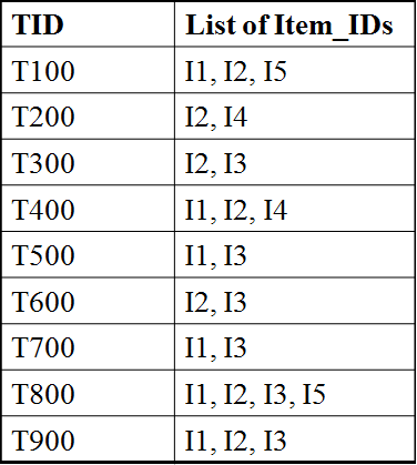
Problem 2: Consider the transaction database, D, which contains 9 records.
The set of items, I = {I1, I2, I3, I4, I5}.
Assume minimum support, s = 22%. Illustrate the working of Apriori algorithm for the database D. And also generate the strong association rules for minimum condfidence (min_conf), c = 80%.
Solution:
Since s = 22% and D contains 9 records.
So, minimum support count value is = (9×22)/100 = 1.98 ≈ 2.
k := 1
C1
Itemset Support count
{I1} 6
{I2} 7
{I3} 6
{I4} 2
{I5} 2
L1
Itemset Support count
{I1} 6
{I2} 7
{I3} 6
{I4} 2
{I5} 2
k := 2
C2
Itemset Support count
{I1, I2} 4
{I1, I3} 4
{I1, I4} 1
{I1, I5} 2
{I2, I3} 4
{I2, I4} 2
{I2, I5} 2
{I3, I4} 0
{I3, I5} 1
{I4, I5} 0
L2
Itemset Support count
{I1, I2} 4
{I1, I3} 4
{I1, I5} 2
{I2, I3} 4
{I2, I4} 2
{I2, I5} 2
k := 3
C3
Itemset Support count
{I1, I2, I3} 2
{I1, I2, I5} 2
{I1, I3, I5} X
{I2, I3, I4} X
{I2, I3, I5} X
{I2, I4, I5} X
[‘X‘ denotes the use of Apriori property to prune itemsets]
L3
Itemset Support count
{I1, I2, I3} 2
{I1, I2, I5} 2
k := 4
C4 = { {I1, I2, I3, I5} }
L4 = Ø
L := L1 U L2 U L3
Now, based on the definition of confidence threshold, association rules can be generated as follows:
♦ for each frequent itemset l, generate all nonempty subsets of l.
♦ for every nonempty subset s of l, output the rule “s ⇒ (l – s)” if support_count(s) / support_count(l) ≥ min_conf
Let us consider the 3-itemset {I1, I2, I5} with support of 2 (22)%. Let’s generate all the association rules from this itemset:
I1 ∧ I2 ⇒ I5, confidence= 2/4 = 50%
I1 ∧ I5 ⇒ I2, confidence= 2/2 = 100%
I2 ∧ I5 ⇒ I1, confidence= 2/2 = 100%
I1 ⇒ I2 ∧ I5, confidence= 2/6 = 33%
I2 ⇒ I1 ∧ I5, confidence= 2/7 = 29%
I5 ⇒ I1 ∧ I2, confidence= 2/2 = 100%
If the minimum confidence threshold, c is 80%, then only the second, third, and last rules above are output, because these are the only ones generated that are strong.