Other Important Classifiers

Apart from ANN, DT and SVM, there are some important classifiers which worth mentioning. For example, K-Nearest Neighbor (K-NN), Naive Bayes, Logistic Regression, Random Forest etc. are well-known classifiers in the classification domain. They are described below in brief. We also give here the Python code snippet (i.e. part of a code) for each of the classifiers which is to applied on the preprocessed dataset.

K-Nearest Neighbor (K-NN)

The K-Nearest Neighbor (K-NN) is an instance-based learning method for classifying objects using the rationale of nearest training examples within the search space. The procedure compares a given test pattern with training patterns that are similar to it. One should use suitable distance metric to assign a new data point to the most frequently occurring class in the neighborhood. The distance metric used in this approach may be the Euclidean distance to select the nearest neighbors.

The Euclidean distance between points p and q is the length of the line segment connecting them $\overline{\mathbf{p}\mathbf{q}}$ .

In Cartesian coordinates, if p = (p₁, p₂,…, p_n) and q = (q₁, q₂,…, q_n) are two points in Euclidean n-space, then the Euclidean distance (d) from p to q, or from q to p is given by the Pythagorean formula:

${\begin{aligned}d(\mathbf {p} ,\mathbf {q} )=d(\mathbf {q} ,\mathbf {p} )&={\sqrt {(q_{1}-p_{1})^{2}+(q_{2}-p_{2})^{2}+\cdots +(q_{n}-p_{n})^{2}}}\\[8pt]&={\sqrt {\sum _{i=1}^{n}(q_{i}-p_{i})^{2}}}.\end{aligned}}$

Let us consider a simple K-NN example with K = 7 and a given query-instance x_q as shown in Figure 1 below. Initially, after selecting the value of K, we have to compute the distance between the query-instance and all training tuples using a distance metric (for example, Euclidean distance). Then we sort the distances for all training tuples and find the nearest neighbor to K — the minimum distance. After that we have to determine all the categories of the training data for the sorted value that fall under k. In this case, the query-instance x_q will be classified as ‘–’ (negative) since four of its nearest neighbors are marked as ‘–’ . This classification procedure is based solely on majority voting by its nearest neighbors.

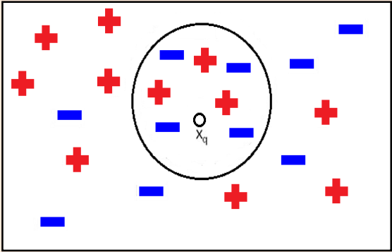
Figure 1: A k-NN example with k=7

Python code snippet for K-NN:

# Import the library
from sklearn.neighbors import KNeighborsClassifier

# Training the model
model = KNeighborsClassifier()

Naive Bayes

The Naive Bayes is a statistical classifier. It can predict class membership probabilities, such as the probability that a given tuple belongs to a particular class. Bayesian classification follows Bayes’ theorem which is based on the concept of conditional probability.

Bayes’s theorem is stated mathematically as the following equation:

P(A|B) = P(A) P(B|A) / P(B) ———> (2)

where $A$ and $B$ are events and $P(B)\neq 0$ .

$P(A\mid B)$ is a conditional probability: the likelihood of $A$ occurring given that $B$ is true.
$P(B\mid A)$ is a conditional probability: the likelihood of $B$ occurring given that $A$ is true.
$P(A)$ and $P(B)$ are the probabilities of observing $A$ and $B$ respectively

Naive Bayesian classifier is comparable in performance with decision tree and selected neural network classifiers. It has also exhibited high accuracy and speed when applied to large databases.

Python code snippet for Naive Bayes:

# Import the library
from sklearn.naive_bayes import GaussianNB

# Training the model
model = GaussianNB()

Logistic Regression

Generalized linear models represent the theoretical foundation on which linear regression can be applied to the modeling of categorical dependent variables (i.e. categorical response variables). In generalized linear models, the variance of the dependent variable, Y, is a function of the mean value of Y, unlike in linear regression, where the variance of Y is constant. Common types of generalized linear models include logistic regression.

Logistic regression models the probability of some event occurring as a linear function of a set of independent variables (i.e. predictor variables). It forecasts the probability of an outcome that is having binary values (e.g. 0/1 or Y/N). This technique is used when the dependent variable (i.e. target variable) is categorical.

Logistic regression is different from linear regression because of the logit function. As Y is a binary response variable, we use the logit of probability p as the response in the regression equation instead of just Y, which we denote p = P(Y = 1).

We assume a linear relationship between the predictor variables and the log-odds (i.e. the logarithm of the odds) of the event that Y = 1. This linear relationship can be written in the following mathematical form (where ℓ is the log-odds, and β_i are the parameters of the model):

ℓ = log[p / (1 – p)] = β₀ + β₁x₁ + β₂x₂ + … + β_kx_k

where p is the probability of presence of the characteristic of interest (i.e. Y = 1) given by:

p = 1 / [1 + e^{−(β₀ + β₁x₁ + β₂x₂ + … + β_kx_k)}]

The log-odds are defined as:

odds = p / (1 – p) = probability of presence / probability of absence

and the logarithm of the odds is the logit of the probability defined as follows:

logit(p) = log[p / (1 – p)] for

0 < p <1

The regression coefficients are estimated using iteratively re-weighted least squares method or maximum likelihood estimation rather than ordinary least square method and works better with large sample sizes.

Python code snippet for Logistic regression:

# Import the library
from sklearn.linear_model import LogisticRegression

# Training the model
model = LogisticRegression()

Random Forest (RF)

Random Forest (RF) is based on the supervised classification algorithm. RF makes predictions by combining the results from many individual decision trees – so we can call them a forest of decision trees. Because RF combines multiple models, it falls under the category of ensemble learning. Commonly used ensemble learning algorithms are bagging and boosting.

Basically, RF classifier tries to create a forest by using bagging (also called Bootstrap aggregation) and makes it random. There is a direct relationship between the number of trees in the forest and the results it can get: the larger the number of trees, the more accurate the result.

In essence, RF creates multiple decision trees based on input data samples and then gets the prediction from each of them and finally selects the best solution by means of majority voting. It is better than a single decision tree because it reduces the over-fitting by averaging the result. The process is described below in Figure 2.

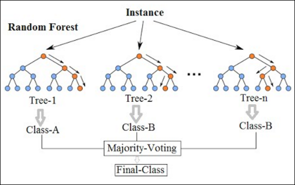
Figure 2: A sample Random Forest created using multiple decision trees

Python code snippet for Random Forest:

# Import the library
from sklearn.ensemble import RandomForestClassifier

# Training the model
model = RandomForestClassifier()

⇒ N.B. We have given here code snippets to mention the classifier names and their corresponding Python module names only. For complete implementation of these classifiers you have to go through the previous tutorial involving MLP, DT, and SVM models.

In the next tutorial, I will discuss about Regression Technique.