Decision Tree (DT)
Decision Tree (DT) is a classification model in which a decision tree learns from the tuples in the training dataset. A decision tree appears like a flowchart in a tree like structure, where each internal node denotes condition testing on an attribute, each branch resulting from that node denotes the outcome from the test. The leaf node in the decision tree holds a class label. In this tree, the nodes divide the tuples into different groups at each level of the tree until they fall into distinct class labels. A sample decision tree is illustrated in Figure 1.
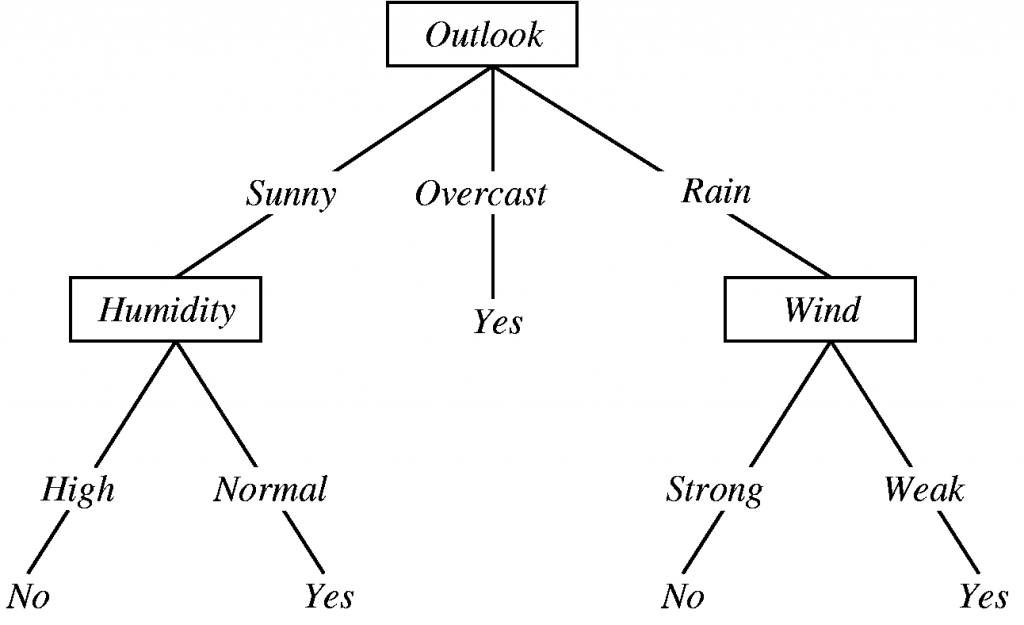
Figure 1: A sample decision tree classifier
There are three commonly known variations of decision tree algorithms. They are given as follows:
- ID3 (Iterative Dichotomiser)
- C4.5
- CART (Classification and Regression Trees)
ID3, C4.5 and CART are developed using greedy approach. Most of these methods follow a top-down approach, in which the tree starts with a set of tuples and their corresponding classes. The tree starts with a single node containing all the tuples. If all the tuples are in the same class then this becomes the leaf node and the tree is not further divided. Otherwise, the set of tuples is divided into two or more parts in accordance with the splitting criterion.
The splitting criterion involves splitting of the set of tuples into subsets in correspondence to the grouping done with respect to the splitting attribute. The splitting criterion is chosen in such a way that the tuples are grouped in the best possible way. If a node is marked with the splitting criterion then branches are created for each outcome of the test. Using this principle recursively the learning decision tree is built.
An attribute selection needs to be done for obtaining the best splitting criterion that can correctly and accurately separate the tuples into classes. This attribute selection method (also called splitting rules) determines hoe the tuples are to be divided. The attribute having the best score is selected as the splitting attribute. There are three popular attribute selection measures — information gain, gain ratio and gini index. They are described below.
1. Information Gain
The attribute selection measure for the ID3 algorithm is the information gain. Let D be the training data set consisting of class-labeled tuples. Suppose the class label attribute has m distinct values describing m distinct classes, Ci (for i = 1, 2, 3, …., m). Let Ci,D be the set of tuples of class Ci in D. Let |Dj| and |Ci,D| denote the number of tuples in D and Ci,D, respectively. The expected information needed to classify a tuple in D is given by:
Info(D) = – ∑i pi log2 (pi) ———> (1) [for i = 1, 2, …, m]
where pi is the probability that a random tuple in D fits in class Ci and is assessed by the ratio |Ci,D|/|D|.
Now, suppose the procedure are to divide the tuples in D on some attribute A having v different values, (a1, a2, …, av), as detected from the training data set. If A is discrete-valued, these values relate directly to the v outcomes of a test on A. Attribute A can be used to split D into v divisions or subsets, (D1, D2, … , Dv), where Dj comprises those tuples in D that have outcome aj of A.
InfoA(D) = – ∑j (|Dj|/|D|) × Info(Dj) ———> (2) [for j = 1, 2, …, v]
Information gain is defined as the difference between the original information constraint (i.e., based on the proportion of data classes) and the new constraint (i.e., obtained after dividing on A). That is,
Gain(A) = Info(D) – InfoA(D) ———> (3)
The attribute A with the highest information gain is selected as the splitting attribute.
2. Gain Ratio
The information gain metric is biased toward tests with many outcomes. Basically, it prefers to select attributes having a large number of values. That is why another term has been introduced which is known as the gain ratio. C4.5, a successor of ID3, uses the concept of gain ratio to avoid this bias. It applies a kind of normalization to information gain using a “split information” value defined analogously with Info(D) as:
SplitInfoA(D) = – ∑j (|Dj|/|D|) × log2(|Dj|/|D|) ———> (4) [for j = 1, 2, …, v]
This value denotes the probable information produced by splitting the training data set, D, into v divisions, conforming to the v results of a test on attribute A. Hence, the gain ratio is defined as:
GainRatio(A) = Gain(A) / SplitInfo(A) ———> (5)
Typically, the attribute with the largest gain ratio is designated as the splitting attribute.
3. Gini Index
The third algorithm is known as Classification and Regression Trees (CART). Basically, we select CART to avoid a situation where split information tends to zero and the gain ratio becomes unstable which can affect the performance of the classification model. CART uses Gini index for selection of attribute. The Gini index is based upon the amount of impurity content in a set of tuples D. This can be represented as:
Gini(D) = 1 – ∑i pi2 ———> (6) [for i = 1, 2, …, m]
where pi is the probability that a tuple that belong to D falls under an arbitrary class Ci. This is done for a range of m classes. Binary splitting is done for each attribute in Gini index. For splitting on the attribute A, we consider two partitions D1 and D2 from D, the Gini index of the partitioning can be given as:
GiniA(D) = (|D1|/|D|) Gini(D1) + (|D2|/|D|) Gini(D2) ———> (7)
All possible combination of partitions is considered for each attribute A in the given data. The subset that gives the minimum Gini index is selected as the splitting subset. After this selection we need to calculate the amount of impurity present after the occurrence of binary splitting. This can be calculated as:
Gini(A) = Gini(A) – GiniA(D) ———> (8)
The attribute which has the maximum reduction of impurity after splitting is selected. This attribute is selected as the splitting attribute for splitting in CART.
Basically, CART algorithm uses the concept of “binary split”. Here, the attribute with the smallest Gini index is designated as the splitting attribute.