Case Study – k-Means
k-Means clustering algorithm creates various partitions and then evaluate them by using the concept of minimizing the within-cluster sum of squares (WCSS). The input to this algorithm is the number of data objects present in the dataset (say n) and the number of clusters (say k) to be specified by the user. The output of the algorithm is the set of k clusters resulting in high intra-cluster similarity but low inter-cluster similarity.
Dataset Description
For implementation of k-Means algorithm we will use the Iris dataset of UCI. This dataset contains 3 classes of 50 instances each and each class refers to a type of Iris plant. The dataset has four input features: sepal length, sepal width, petal length, and petal width (all the units are in cm). The fifth column is for class label, which holds the species information for these types of plants. As because we are implementing k-Means clustering algorithm, we can understand that the class label column is not needed for this experiment.
k-Means Implementation
In this section, we will use the Iris dataset to demonstrate the k-Means clustering algorithm based on the four input features: sepal length, sepal width, petal length, and petal width. We will follow here step-by-step approach (with code and output of intermediate step) to demonstrate this algorithm. The Python code statements are run using IPython console.
Step 1: Import the libraries
import pandas as pd
import numpy as np
import matplotlib.pyplot as plt
from sklearn.cluster import KMeans
Step 2: Load the dataset and display statistics
df = pd.read_csv('iris.csv')
print(df.shape) # shape
print(df.head(10)) # first 10 records
print(df.describe()) # descriptions
Output:
(150, 5)
   sepal length  sepal width     ...       petal width        class
0           5.1          3.5     ...               0.2  Iris-setosa
1           4.9          3.0     ...               0.2  Iris-setosa
2           4.7          3.2     ...               0.2  Iris-setosa
3           4.6          3.1     ...               0.2  Iris-setosa
4           5.0          3.6     ...               0.2  Iris-setosa
5           5.4          3.9     ...               0.4  Iris-setosa
6           4.6          3.4     ...               0.3  Iris-setosa
7           5.0          3.4     ...               0.2  Iris-setosa
8           4.4          2.9     ...               0.2  Iris-setosa
9           4.9          3.1     ...               0.1  Iris-setosa

[10 rows x 5 columns]
       sepal length  sepal width  petal length  petal width
count    150.000000   150.000000    150.000000   150.000000
mean       5.843333     3.054000      3.758667     1.198667
std        0.828066     0.433594      1.764420     0.763161
min        4.300000     2.000000      1.000000     0.100000
25%        5.100000     2.800000      1.600000     0.300000
50%        5.800000     3.000000      4.350000     1.300000
75%        6.400000     3.300000      5.100000     1.800000
max        7.900000     4.400000      6.900000     2.500000
Step 3: Select all four features of the dataset
data = df.iloc[:, [0,1,2,3]].values
Step 4: Develop k-Means model with k=4
To start with, we arbitrarily assign the value of k as 4. Sooner we will discover the optimal value of k. But, for the time being, we implement k-Means clustering using k=4. Using this, we instantiate the KMeans class and assign it to the variable model4:
model4 = KMeans(n_clusters = 4)
result4 = model4.fit_predict(data)
print(result4)
Output:
[1 1 1 1 1 1 1 1 1 1 1 1 1 1 1 1 1 1 1 1 1 1 1 1 1 1 1 1 1 1 1 1 1 1 1 1 1
1 1 1 1 1 1 1 1 1 1 1 1 1 2 2 2 0 2 0 2 0 2 0 0 0 0 2 0 2 0 0 2 0 2 0 2 2
2 2 2 2 2 0 0 0 0 2 0 2 2 2 0 0 0 2 0 0 0 0 0 2 0 0 3 2 3 3 3 3 0 3 3 3 2
2 3 2 2 3 3 3 3 2 3 2 3 2 3 3 2 2 3 3 3 3 3 2 2 3 3 3 2 3 3 3 2 3 3 3 2 2
3 2]
Step 5: Display the cluster centers
centers = model4.cluster_centers_
print(centers)
Output:
[[5.53214286 2.63571429 3.96071429 1.22857143]
[5.006 3.418 1.464 0.244 ]
[6.2525 2.855 4.815 1.625 ]
[6.9125 3.1 5.846875 2.13125 ]]
Step 6: Find optimal value of k using Elbow method
Now, we will employ a method called the Elbow method, to find out the optimal number of clusters in the dataset. To implement this method, we need to develop some Python code here, and we will plot a graph between the number of clusters and the corresponding sum of square errors value.
To get the values used in the graph, we train multiple models using a different number of clusters and storing the value of the intertia_ property (WCSS) every time. As the graph generally ends up shaped like an elbow, hence such peculiar name is given to this method:
wcss = []
for i in range(1, 11):
    model = KMeans(n_clusters = i).fit(data)
    model.fit(data)
    wcss.append(model.inertia_)
# plot the graph
plt.plot(range(1, 11), wcss)
plt.title('Elbow method')
plt.xlabel('Number of clusters')
plt.ylabel('WCSS')
plt.show()
Output:
The output graph of the Elbow method is shown below. Note that the shape of elbow is approximately formed at k=3.
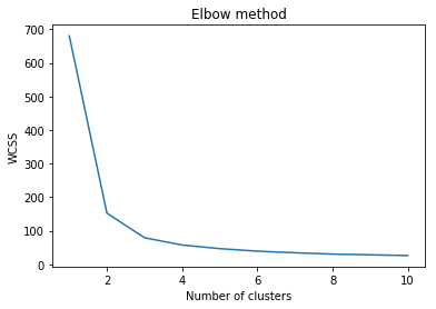
As we can see, the optimal value of k is between 2 and 4, as the elbow-like shape is formed at k=3 in the above graph. So, we will now implement k-Means again using k=3.
Step 7: Develop k-Means model with k=3
model3 = KMeans(n_clusters = 3)
result3 = model3.fit_predict(data)
print(result3)
Output:
[0 0 0 0 0 0 0 0 0 0 0 0 0 0 0 0 0 0 0 0 0 0 0 0 0 0 0 0 0 0 0 0 0 0 0 0 0
0 0 0 0 0 0 0 0 0 0 0 0 0 1 1 2 1 1 1 1 1 1 1 1 1 1 1 1 1 1 1 1 1 1 1 1 1
1 1 1 2 1 1 1 1 1 1 1 1 1 1 1 1 1 1 1 1 1 1 1 1 1 1 2 1 2 2 2 2 1 2 2 2 2
2 2 1 1 2 2 2 2 1 2 1 2 1 2 2 1 1 2 2 2 2 2 1 2 2 2 2 1 2 2 2 1 2 2 2 1 2
2 1]
Step 8: Display the cluster centers for k=3
centers = model3.cluster_centers_
print(centers)
Output:
[[5.006 3.418 1.464 0.244 ]
[5.9016129 2.7483871 4.39354839 1.43387097]
[6.85 3.07368421 5.74210526 2.07105263]]
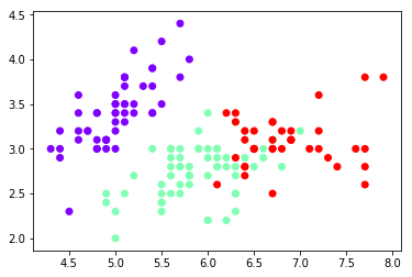
Step 9: Visualize clusters using graphic plot for k=3
Finally, we will visualize the 3 clusters that are formed with the optimal value of k. We can obviously see the presence of the 3 clusters in the image below, with each cluster represented by a different color.
plt.scatter(data[:,0], data[:,1], c=result3, cmap='rainbow')Output:
I hope that now you have got the confidence of solving any kind of clustering problem in the ML domain. It is advisable that you should use the graphic plots regularly to make the output more comprehensible.